
Python Setup
To read National Water Model data you will need the netCDF4 package. To manipulate and plot the data we recommend matplotlib, cartopy, fiona, shapely & numpy.
We have setup a Docker container with a suitably configured Jupyter notebook at https://github.com/occ-data/docker-jupyter.
%matplotlib inline
from netCDF4 import Dataset
import matplotlib
import matplotlib.pyplot as plt
from mpl_toolkits.axes_grid1 import ImageGrid
import numpy as np
from MPLColorHelper import MplColorHelper
import cartopy.crs as ccrs
from cartopy import feature
import fiona
from shapely.geometry import shape, MultiLineString
import boto3
from botocore import UNSIGNED
from botocore.client import Config
import zipfile
import os.path
Download NWM data from the OCC Environmental Data Commons
This assumes we know the file names and date time of the data we want.
- YYYYMMDDHHMM.LDASOUT_DOMAIN1 Land surface model outputs
- YYYYMMDDHHMM.LAKEOUT_DOMAIN1 Lake/Reservoir model outputs
- YYYYMMDDHHMM.GWOUT_DOMAIN1
- YYYYMMDDHHMM.RTOUT_DOMAIN1
- YYYYMMDDHHMM.CHRTOUT_DOMAIN1 Channel model vector outputs
s3 = boto3.client('s3', endpoint_url="https://griffin-objstore.opensciencedatacloud.org",
                  config=Config(signature_version=UNSIGNED))
if not os.path.isfile("201409090000.LDASOUT_DOMAIN1.comp"):
    s3.download_file("nwm-archive", "2014/201409090000.LDASOUT_DOMAIN1.comp", "201409090000.LDASOUT_DOMAIN1.comp")
if not os.path.isfile("201409090000.CHRTOUT_DOMAIN1.comp"):
    s3.download_file("nwm-archive", "2014/201409090000.CHRTOUT_DOMAIN1.comp", "201409090000.CHRTOUT_DOMAIN1.comp")
The NWM data comes in several files per timestep, here we use the land surface model output
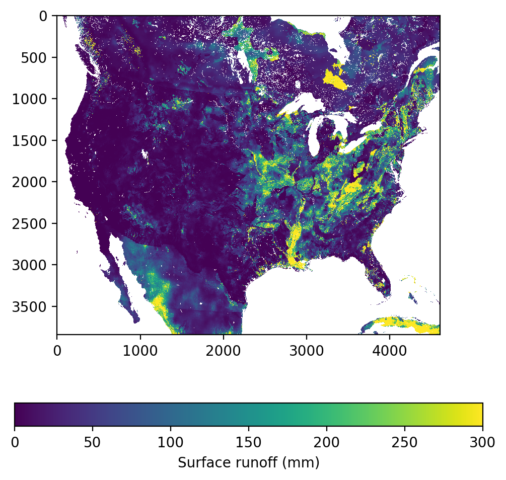
We will look at the volumetric soil moisture, which is computed for 4 separate soil layers, and the surface runoff. We are looking at September 9th, 2014 00:00 UTC, which was in the middle of a significant multi-year California drought. At the time of this data there was also flash flooding occurring in the Phoenix metro area.
First lets see what variables this file has stored.
ldas = Dataset('201409090000.LDASOUT_DOMAIN1.comp', 'r')
ldas_vars = ldas.variables
print(ldas_vars)
OrderedDict([('time', <class 'netCDF4._netCDF4.Variable'>
int32 time(time)
long_name: valid output time
standard_name: time
units: minutes since 1970-01-01 00:00:00 UTC
unlimited dimensions: time
current shape = (1,)
filling on, default _FillValue of -2147483647 used
), ('reference_time', <class 'netCDF4._netCDF4.Variable'>
int32 reference_time(reference_time)
long_name: model initialization time
standard_name: forecast_reference_time
units: minutes since 1970-01-01 00:00:00 UTC
unlimited dimensions:
current shape = (1,)
filling on, default _FillValue of -2147483647 used
), ('x', <class 'netCDF4._netCDF4.Variable'>
float64 x(x)
long_name: x coordinate of projection
standard_name: projection_x_coordinate
_CoordinateAxisType: GeoX
units: m
resolution: 1000.0
unlimited dimensions:
current shape = (4608,)
filling on, default _FillValue of 9.969209968386869e+36 used
), ('y', <class 'netCDF4._netCDF4.Variable'>
float64 y(y)
long_name: y coordinate of projection
standard_name: projection_y_coordinate
_CoordinateAxisType: GeoY
units: m
resolution: 1000.0
unlimited dimensions:
current shape = (3840,)
filling on, default _FillValue of 9.969209968386869e+36 used
), ('ProjectionCoordinateSystem', <class 'netCDF4._netCDF4.Variable'>
|S1 ProjectionCoordinateSystem()
_CoordinateTransformType: Projection
transform_name: lambert_conformal_conic
grid_mapping_name: lambert_conformal_conic
_CoordinateAxes: y x
esri_pe_string: PROJCS["Sphere_Lambert_Conformal_Conic",GEOGCS["GCS_Sphere",DATUM["D_Sphere",SPHEROID["Sphere",6370000.0,0.0]],PRIMEM["Greenwich",0.0],UNIT["Degree",0.0174532925199433]],PROJECTION["Lambert_Conformal_Conic"],PARAMETER["false_easting",0.0],PARAMETER["false_northing",0.0],PARAMETER["central_meridian",-97.0],PARAMETER["standard_parallel_1",30.0],PARAMETER["standard_parallel_2",60.0],PARAMETER["latitude_of_origin",40.000008],UNIT["Meter",1.0]];-35691800 -29075200 126180232.640845;-100000 10000;-100000 10000;0.001;0.001;0.001;IsHighPrecision
standard_parallel: [30. 60.]
longitude_of_central_meridian: -97.0
latitude_of_projection_origin: 40.00000762939453
false_easting: 0.0
false_northing: 0.0
earth_radius: 6370000.0
proj4: +proj=lcc +lat_1=30 +lat_2=60 +lat_0=40 +lon_0=-97 +x_0=0 +y_0=0 +a=6370000 +b=6370000 +units=m +no_defs
unlimited dimensions:
current shape = ()
filling on, default _FillValue of � used
), ('FSA', <class 'netCDF4._netCDF4.Variable'>
int32 FSA(time, y, x)
_FillValue: -99990
missing_value: -99990
long_name: Total absorved SW radiation
units: W m-2
scale_factor: 0.1
add_offset: 0.0
valid_range: [-15000 15000]
proj4: +proj=lcc +lat_1=30 +lat_2=60 +lat_0=40 +lon_0=-97 +x_0=0 +y_0=0 +a=6370000 +b=6370000 +units=m +no_defs
grid_mapping: ProjectionCoordinateSystem
esri_pe_string: PROJCS["Sphere_Lambert_Conformal_Conic",GEOGCS["GCS_Sphere",DATUM["D_Sphere",SPHEROID["Sphere",6370000.0,0.0]],PRIMEM["Greenwich",0.0],UNIT["Degree",0.0174532925199433]],PROJECTION["Lambert_Conformal_Conic"],PARAMETER["false_easting",0.0],PARAMETER["false_northing",0.0],PARAMETER["central_meridian",-97.0],PARAMETER["standard_parallel_1",30.0],PARAMETER["standard_parallel_2",60.0],PARAMETER["latitude_of_origin",40.000008],UNIT["Meter",1.0]];-35691800 -29075200 126180232.640845;-100000 10000;-100000 10000;0.001;0.001;0.001;IsHighPrecision
unlimited dimensions: time
current shape = (1, 3840, 4608)
filling on), ('FIRA', <class 'netCDF4._netCDF4.Variable'>
int32 FIRA(time, y, x)
_FillValue: -99990
missing_value: -99990
long_name: Total net LW radiation to atmosphere
units: W m-2
scale_factor: 0.1
add_offset: 0.0
valid_range: [-15000 15000]
proj4: +proj=lcc +lat_1=30 +lat_2=60 +lat_0=40 +lon_0=-97 +x_0=0 +y_0=0 +a=6370000 +b=6370000 +units=m +no_defs
grid_mapping: ProjectionCoordinateSystem
esri_pe_string: PROJCS["Sphere_Lambert_Conformal_Conic",GEOGCS["GCS_Sphere",DATUM["D_Sphere",SPHEROID["Sphere",6370000.0,0.0]],PRIMEM["Greenwich",0.0],UNIT["Degree",0.0174532925199433]],PROJECTION["Lambert_Conformal_Conic"],PARAMETER["false_easting",0.0],PARAMETER["false_northing",0.0],PARAMETER["central_meridian",-97.0],PARAMETER["standard_parallel_1",30.0],PARAMETER["standard_parallel_2",60.0],PARAMETER["latitude_of_origin",40.000008],UNIT["Meter",1.0]];-35691800 -29075200 126180232.640845;-100000 10000;-100000 10000;0.001;0.001;0.001;IsHighPrecision
unlimited dimensions: time
current shape = (1, 3840, 4608)
filling on), ('HFX', <class 'netCDF4._netCDF4.Variable'>
int32 HFX(time, y, x)
_FillValue: -99990
missing_value: -99990
long_name: Total sensible heat to the atmosphere
units: W m-2
scale_factor: 0.1
add_offset: 0.0
valid_range: [-15000 15000]
proj4: +proj=lcc +lat_1=30 +lat_2=60 +lat_0=40 +lon_0=-97 +x_0=0 +y_0=0 +a=6370000 +b=6370000 +units=m +no_defs
grid_mapping: ProjectionCoordinateSystem
esri_pe_string: PROJCS["Sphere_Lambert_Conformal_Conic",GEOGCS["GCS_Sphere",DATUM["D_Sphere",SPHEROID["Sphere",6370000.0,0.0]],PRIMEM["Greenwich",0.0],UNIT["Degree",0.0174532925199433]],PROJECTION["Lambert_Conformal_Conic"],PARAMETER["false_easting",0.0],PARAMETER["false_northing",0.0],PARAMETER["central_meridian",-97.0],PARAMETER["standard_parallel_1",30.0],PARAMETER["standard_parallel_2",60.0],PARAMETER["latitude_of_origin",40.000008],UNIT["Meter",1.0]];-35691800 -29075200 126180232.640845;-100000 10000;-100000 10000;0.001;0.001;0.001;IsHighPrecision
unlimited dimensions: time
current shape = (1, 3840, 4608)
filling on), ('LH', <class 'netCDF4._netCDF4.Variable'>
int32 LH(time, y, x)
_FillValue: -99990
missing_value: -99990
long_name: Total latent heat to the atmosphere
units: W m-2
scale_factor: 0.1
add_offset: 0.0
valid_range: [-15000 15000]
proj4: +proj=lcc +lat_1=30 +lat_2=60 +lat_0=40 +lon_0=-97 +x_0=0 +y_0=0 +a=6370000 +b=6370000 +units=m +no_defs
grid_mapping: ProjectionCoordinateSystem
esri_pe_string: PROJCS["Sphere_Lambert_Conformal_Conic",GEOGCS["GCS_Sphere",DATUM["D_Sphere",SPHEROID["Sphere",6370000.0,0.0]],PRIMEM["Greenwich",0.0],UNIT["Degree",0.0174532925199433]],PROJECTION["Lambert_Conformal_Conic"],PARAMETER["false_easting",0.0],PARAMETER["false_northing",0.0],PARAMETER["central_meridian",-97.0],PARAMETER["standard_parallel_1",30.0],PARAMETER["standard_parallel_2",60.0],PARAMETER["latitude_of_origin",40.000008],UNIT["Meter",1.0]];-35691800 -29075200 126180232.640845;-100000 10000;-100000 10000;0.001;0.001;0.001;IsHighPrecision
unlimited dimensions: time
current shape = (1, 3840, 4608)
filling on), ('UGDRNOFF', <class 'netCDF4._netCDF4.Variable'>
int32 UGDRNOFF(time, y, x)
_FillValue: -999900
missing_value: -999900
long_name: Accumulated underground runoff
units: mm
scale_factor: 0.01
add_offset: 0.0
valid_range: [ -500 3000000]
proj4: +proj=lcc +lat_1=30 +lat_2=60 +lat_0=40 +lon_0=-97 +x_0=0 +y_0=0 +a=6370000 +b=6370000 +units=m +no_defs
grid_mapping: ProjectionCoordinateSystem
esri_pe_string: PROJCS["Sphere_Lambert_Conformal_Conic",GEOGCS["GCS_Sphere",DATUM["D_Sphere",SPHEROID["Sphere",6370000.0,0.0]],PRIMEM["Greenwich",0.0],UNIT["Degree",0.0174532925199433]],PROJECTION["Lambert_Conformal_Conic"],PARAMETER["false_easting",0.0],PARAMETER["false_northing",0.0],PARAMETER["central_meridian",-97.0],PARAMETER["standard_parallel_1",30.0],PARAMETER["standard_parallel_2",60.0],PARAMETER["latitude_of_origin",40.000008],UNIT["Meter",1.0]];-35691800 -29075200 126180232.640845;-100000 10000;-100000 10000;0.001;0.001;0.001;IsHighPrecision
unlimited dimensions: time
current shape = (1, 3840, 4608)
filling on), ('SFCRNOFF', <class 'netCDF4._netCDF4.Variable'>
int32 SFCRNOFF(time, y, x)
_FillValue: -9999000
missing_value: -9999000
long_name: Accumulated surface runoff
units: mm
scale_factor: 0.001
add_offset: 0.0
valid_range: [ 0 29999998]
proj4: +proj=lcc +lat_1=30 +lat_2=60 +lat_0=40 +lon_0=-97 +x_0=0 +y_0=0 +a=6370000 +b=6370000 +units=m +no_defs
grid_mapping: ProjectionCoordinateSystem
esri_pe_string: PROJCS["Sphere_Lambert_Conformal_Conic",GEOGCS["GCS_Sphere",DATUM["D_Sphere",SPHEROID["Sphere",6370000.0,0.0]],PRIMEM["Greenwich",0.0],UNIT["Degree",0.0174532925199433]],PROJECTION["Lambert_Conformal_Conic"],PARAMETER["false_easting",0.0],PARAMETER["false_northing",0.0],PARAMETER["central_meridian",-97.0],PARAMETER["standard_parallel_1",30.0],PARAMETER["standard_parallel_2",60.0],PARAMETER["latitude_of_origin",40.000008],UNIT["Meter",1.0]];-35691800 -29075200 126180232.640845;-100000 10000;-100000 10000;0.001;0.001;0.001;IsHighPrecision
unlimited dimensions: time
current shape = (1, 3840, 4608)
filling on), ('TRAD', <class 'netCDF4._netCDF4.Variable'>
int32 TRAD(time, y, x)
_FillValue: -99990
missing_value: -99990
long_name: Surface radiative temperature
units: K
scale_factor: 0.1
add_offset: 0.0
valid_range: [-10000 10000]
proj4: +proj=lcc +lat_1=30 +lat_2=60 +lat_0=40 +lon_0=-97 +x_0=0 +y_0=0 +a=6370000 +b=6370000 +units=m +no_defs
grid_mapping: ProjectionCoordinateSystem
esri_pe_string: PROJCS["Sphere_Lambert_Conformal_Conic",GEOGCS["GCS_Sphere",DATUM["D_Sphere",SPHEROID["Sphere",6370000.0,0.0]],PRIMEM["Greenwich",0.0],UNIT["Degree",0.0174532925199433]],PROJECTION["Lambert_Conformal_Conic"],PARAMETER["false_easting",0.0],PARAMETER["false_northing",0.0],PARAMETER["central_meridian",-97.0],PARAMETER["standard_parallel_1",30.0],PARAMETER["standard_parallel_2",60.0],PARAMETER["latitude_of_origin",40.000008],UNIT["Meter",1.0]];-35691800 -29075200 126180232.640845;-100000 10000;-100000 10000;0.001;0.001;0.001;IsHighPrecision
unlimited dimensions: time
current shape = (1, 3840, 4608)
filling on), ('SOIL_W', <class 'netCDF4._netCDF4.Variable'>
int32 SOIL_W(time, y, soil_layers_stag, x)
_FillValue: -999900
missing_value: -999900
long_name: liquid volumetric soil moisture
units: m3 m-3
scale_factor: 0.01
add_offset: 0.0
valid_range: [ 0 100]
proj4: +proj=lcc +lat_1=30 +lat_2=60 +lat_0=40 +lon_0=-97 +x_0=0 +y_0=0 +a=6370000 +b=6370000 +units=m +no_defs
grid_mapping: ProjectionCoordinateSystem
esri_pe_string: PROJCS["Sphere_Lambert_Conformal_Conic",GEOGCS["GCS_Sphere",DATUM["D_Sphere",SPHEROID["Sphere",6370000.0,0.0]],PRIMEM["Greenwich",0.0],UNIT["Degree",0.0174532925199433]],PROJECTION["Lambert_Conformal_Conic"],PARAMETER["false_easting",0.0],PARAMETER["false_northing",0.0],PARAMETER["central_meridian",-97.0],PARAMETER["standard_parallel_1",30.0],PARAMETER["standard_parallel_2",60.0],PARAMETER["latitude_of_origin",40.000008],UNIT["Meter",1.0]];-35691800 -29075200 126180232.640845;-100000 10000;-100000 10000;0.001;0.001;0.001;IsHighPrecision
unlimited dimensions: time
current shape = (1, 3840, 4, 4608)
filling on), ('SOIL_M', <class 'netCDF4._netCDF4.Variable'>
int32 SOIL_M(time, y, soil_layers_stag, x)
_FillValue: -999900
missing_value: -999900
long_name: volumetric soil moisture
units: m3 m-3
scale_factor: 0.01
add_offset: 0.0
valid_range: [ 0 100]
proj4: +proj=lcc +lat_1=30 +lat_2=60 +lat_0=40 +lon_0=-97 +x_0=0 +y_0=0 +a=6370000 +b=6370000 +units=m +no_defs
grid_mapping: ProjectionCoordinateSystem
esri_pe_string: PROJCS["Sphere_Lambert_Conformal_Conic",GEOGCS["GCS_Sphere",DATUM["D_Sphere",SPHEROID["Sphere",6370000.0,0.0]],PRIMEM["Greenwich",0.0],UNIT["Degree",0.0174532925199433]],PROJECTION["Lambert_Conformal_Conic"],PARAMETER["false_easting",0.0],PARAMETER["false_northing",0.0],PARAMETER["central_meridian",-97.0],PARAMETER["standard_parallel_1",30.0],PARAMETER["standard_parallel_2",60.0],PARAMETER["latitude_of_origin",40.000008],UNIT["Meter",1.0]];-35691800 -29075200 126180232.640845;-100000 10000;-100000 10000;0.001;0.001;0.001;IsHighPrecision
unlimited dimensions: time
current shape = (1, 3840, 4, 4608)
filling on), ('SNOWH', <class 'netCDF4._netCDF4.Variable'>
int32 SNOWH(time, y, x)
_FillValue: -9999000
missing_value: -9999000
long_name: Snow depth
units: m
scale_factor: 0.001
add_offset: 0.0
valid_range: [ 0 99999992]
proj4: +proj=lcc +lat_1=30 +lat_2=60 +lat_0=40 +lon_0=-97 +x_0=0 +y_0=0 +a=6370000 +b=6370000 +units=m +no_defs
grid_mapping: ProjectionCoordinateSystem
esri_pe_string: PROJCS["Sphere_Lambert_Conformal_Conic",GEOGCS["GCS_Sphere",DATUM["D_Sphere",SPHEROID["Sphere",6370000.0,0.0]],PRIMEM["Greenwich",0.0],UNIT["Degree",0.0174532925199433]],PROJECTION["Lambert_Conformal_Conic"],PARAMETER["false_easting",0.0],PARAMETER["false_northing",0.0],PARAMETER["central_meridian",-97.0],PARAMETER["standard_parallel_1",30.0],PARAMETER["standard_parallel_2",60.0],PARAMETER["latitude_of_origin",40.000008],UNIT["Meter",1.0]];-35691800 -29075200 126180232.640845;-100000 10000;-100000 10000;0.001;0.001;0.001;IsHighPrecision
unlimited dimensions: time
current shape = (1, 3840, 4608)
filling on), ('SNEQV', <class 'netCDF4._netCDF4.Variable'>
int32 SNEQV(time, y, x)
_FillValue: -99990
missing_value: -99990
long_name: Snow water equivalent
units: kg m-2
scale_factor: 0.1
add_offset: 0.0
valid_range: [ 0 1000000]
proj4: +proj=lcc +lat_1=30 +lat_2=60 +lat_0=40 +lon_0=-97 +x_0=0 +y_0=0 +a=6370000 +b=6370000 +units=m +no_defs
grid_mapping: ProjectionCoordinateSystem
esri_pe_string: PROJCS["Sphere_Lambert_Conformal_Conic",GEOGCS["GCS_Sphere",DATUM["D_Sphere",SPHEROID["Sphere",6370000.0,0.0]],PRIMEM["Greenwich",0.0],UNIT["Degree",0.0174532925199433]],PROJECTION["Lambert_Conformal_Conic"],PARAMETER["false_easting",0.0],PARAMETER["false_northing",0.0],PARAMETER["central_meridian",-97.0],PARAMETER["standard_parallel_1",30.0],PARAMETER["standard_parallel_2",60.0],PARAMETER["latitude_of_origin",40.000008],UNIT["Meter",1.0]];-35691800 -29075200 126180232.640845;-100000 10000;-100000 10000;0.001;0.001;0.001;IsHighPrecision
unlimited dimensions: time
current shape = (1, 3840, 4608)
filling on), ('FSNO', <class 'netCDF4._netCDF4.Variable'>
int32 FSNO(time, y, x)
_FillValue: -9999000
missing_value: -9999000
long_name: Snow-cover fraction on the ground
units: -
scale_factor: 0.001
add_offset: 0.0
valid_range: [ 0 1000]
proj4: +proj=lcc +lat_1=30 +lat_2=60 +lat_0=40 +lon_0=-97 +x_0=0 +y_0=0 +a=6370000 +b=6370000 +units=m +no_defs
grid_mapping: ProjectionCoordinateSystem
esri_pe_string: PROJCS["Sphere_Lambert_Conformal_Conic",GEOGCS["GCS_Sphere",DATUM["D_Sphere",SPHEROID["Sphere",6370000.0,0.0]],PRIMEM["Greenwich",0.0],UNIT["Degree",0.0174532925199433]],PROJECTION["Lambert_Conformal_Conic"],PARAMETER["false_easting",0.0],PARAMETER["false_northing",0.0],PARAMETER["central_meridian",-97.0],PARAMETER["standard_parallel_1",30.0],PARAMETER["standard_parallel_2",60.0],PARAMETER["latitude_of_origin",40.000008],UNIT["Meter",1.0]];-35691800 -29075200 126180232.640845;-100000 10000;-100000 10000;0.001;0.001;0.001;IsHighPrecision
unlimited dimensions: time
current shape = (1, 3840, 4608)
filling on), ('ACCET', <class 'netCDF4._netCDF4.Variable'>
int32 ACCET(time, y, x)
_FillValue: -999900
missing_value: -999900
long_name: Accumulated total ET
units: mm
scale_factor: 0.01
add_offset: 0.0
valid_range: [-100000 1000000]
proj4: +proj=lcc +lat_1=30 +lat_2=60 +lat_0=40 +lon_0=-97 +x_0=0 +y_0=0 +a=6370000 +b=6370000 +units=m +no_defs
grid_mapping: ProjectionCoordinateSystem
esri_pe_string: PROJCS["Sphere_Lambert_Conformal_Conic",GEOGCS["GCS_Sphere",DATUM["D_Sphere",SPHEROID["Sphere",6370000.0,0.0]],PRIMEM["Greenwich",0.0],UNIT["Degree",0.0174532925199433]],PROJECTION["Lambert_Conformal_Conic"],PARAMETER["false_easting",0.0],PARAMETER["false_northing",0.0],PARAMETER["central_meridian",-97.0],PARAMETER["standard_parallel_1",30.0],PARAMETER["standard_parallel_2",60.0],PARAMETER["latitude_of_origin",40.000008],UNIT["Meter",1.0]];-35691800 -29075200 126180232.640845;-100000 10000;-100000 10000;0.001;0.001;0.001;IsHighPrecision
unlimited dimensions: time
current shape = (1, 3840, 4608)
filling on)])
Now lets load in the volumetric soil moisture and surface runoff. The grids are stored mirrored across the y axis from what we might expect, so we flip them for later plotting purposes too.
VolumetricSoilMoisture = ldas_vars['SOIL_W'][:]
VSM_Layer0 = np.flip(VolumetricSoilMoisture[0,:,0,:], 0)
VSM_Layer1 = np.flip(VolumetricSoilMoisture[0,:,1,:], 0)
VSM_Layer2 = np.flip(VolumetricSoilMoisture[0,:,2,:], 0)
VSM_Layer3 = np.flip(VolumetricSoilMoisture[0,:,3,:], 0)
SurfaceRunoff = ldas_vars['SFCRNOFF'][:]
SurfaceRunoff = np.flip(SurfaceRunoff[0,:,:], 0)
Initial Plots
Lets plot the data first just to see what we are working with here
fig = plt.figure(figsize=(6,6),dpi=200)
im = plt.imshow(SurfaceRunoff, vmin=0.0, vmax=300)
cb = fig.colorbar(im, orientation='horizontal')
cb.set_label('Surface runoff (mm)')
plt.show()
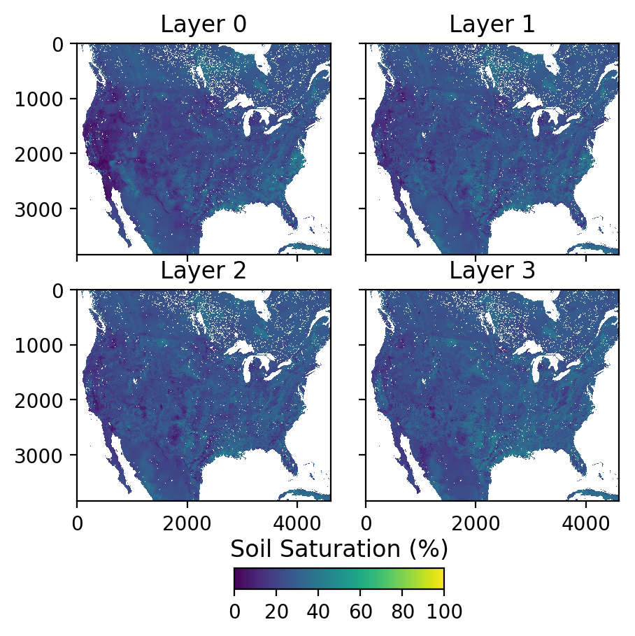
Now lets plot the 4 soil moisture layers so we can compare them.
colorBarMin = 0.0
colorBarMax = 100.0
fig = plt.figure(figsize=(5,5),dpi=200)
grid = ImageGrid(fig, 111,
                 nrows_ncols=(2,2),
                 axes_pad=0.25,
                 share_all=True,
                 )
for ax, a, t in zip(grid, [VSM_Layer0, VSM_Layer1, VSM_Layer2, VSM_Layer3], ["Layer 0", "Layer 1", "Layer 2", "Layer 3"]):
    im = ax.imshow(a * 100.0, vmin=colorBarMin, vmax=colorBarMax)
    ax.set_title(t)

# Legend
ax_legend = fig.add_axes([0.35, 0.05, 0.3, 0.03], zorder=3)
ticks = np.arange(colorBarMin,colorBarMax+0.5,20.0)
cb = matplotlib.colorbar.ColorbarBase(ax_legend, ticks=ticks, norm=matplotlib.colors.Normalize(vmin=colorBarMin, vmax=colorBarMax), orientation='horizontal')
cb.ax.set_xticklabels([str(int(i)) for i in ticks])

plt.title('Soil Saturation (%)')
plt.show()
Vector Stream Plots
The National Water Model has vector based routing using the NHDPlus version 2.1 dataset for the flow network. The information necessary to plot the rivers is not included in the netCDF files but instead must be joined from the NHDPlus database.
To make the data easier to work with, we extract a shapefile for just the flowline network with the attributes we care about. We did this using the GDAL toolset, and specifically the ogr2ogr tool. The commands we used are shown below. We extracted two versions, one which contains only flow lines associated with drainage areas greater than 10,000 square kilometers and the second with flow lines associated with drainage areas greater than 100 square kilometers.
ogr2ogr -f "ESRI Shapefile" -sql "SELECT COMID, TotDASqKm, QA_MA, QC_MA, QE_MA FROM NHDFlowline_Network WHERE TotDASqKm>10000.0" NHDFlowline_Network_Large.shp NHDPlusV21_National_Seamless.gdb
ogr2ogr -f "ESRI Shapefile" -sql "SELECT COMID, TotDASqKm, QA_MA, QC_MA, QE_MA FROM NHDFlowline_Network WHERE TotDASqKm>100.0" NHDFlowline_Network_Small.shp NHDPlusV21_National_Seamless.gdb
This extracts the feature ID so that the vectors in the shapefile can be linked to the netCDF data, the contributing drainage area for each flowline, and some information about the normal expected streamflow values that we will explain later. Here we have extracted the flow lines only for basins above 1,000 km^2. This greatly reduces the file size and makes it easier to demonstrate the techniques here.
The NHDPlusV21 database can be downloaded from http://www.horizon-systems.com/NHDPlusData/NHDPlusV21/Data/NationalData/NHDPlusV21_NationalData_CONUS_Seamless_Geodatabase_05.7z while the document describing what is in this database is at http://www.horizon-systems.com/NHDPlusData/NHDPlusV21/Data/NationalData/NHDPlusV21_National_Seamless_GeoDatabase_User_Guide.pdf
Now lets plot the vector flow network from NHDPlus. Warning: These plots take a very long time to produce.
# Here we load in the shapefiles using fiona

shp_10k = fiona.open('NHDFlowline_Network_Large.shp', 'r')
mp_10k = MultiLineString([shape(line['geometry']) for line in shp_10k])

shp_100 = fiona.open('NHDFlowline_Network_Small.shp', 'r')
mp_100 = MultiLineString([shape(line['geometry']) for line in shp_100])

# The projection is the same for both files so we load it here, just lat-lon coordinates "unprojected"
shpProj = ccrs.PlateCarree()
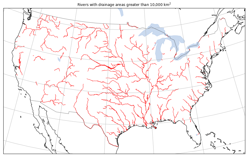
Now that we have the shapefiles loaded in, lets plot the rivers with drainage areas greater than 10,000 km2 to see what that looks like. We use CartoPy for these plots because it is just fast enough to be able to produce them in a reasonable time.
# Define the projection we want to plot our map in here
lccProjParams = { 'central_latitude'   : 50.0, # same as lat_0 in proj4 string
                  'central_longitude'  : -96.0, # same as lon_0
                  'standard_parallels' : (33.0, 45.0) # same as (lat_1, lat_2)
}
proj = ccrs.LambertConformal(**lccProjParams)

fig = plt.figure(figsize=(16,9))
ax = plt.axes(projection = proj)

# Set the visible extent of the map to just CONUS
ax.set_extent([-120.0, -72.0, 22.0, 50.0])

# Plot the rivers we loaded from the shapefile
ax.add_feature(feature.ShapelyFeature(mp_10k, shpProj),
        edgecolor = 'red')


# Additionally plot political borders, lakes and coastlines
# to provide some references on our map
ax.add_feature(feature.NaturalEarthFeature(
        category='cultural',
        name='admin_1_states_provinces_lines',
        scale='50m',
        facecolor='none'))
ax.add_feature(feature.NaturalEarthFeature(
        category='physical',
        name='lakes',
        scale='50m',
        facecolor='none'))
ax.coastlines('50m')
ax.add_feature(feature.LAKES, alpha=0.5)
ax.add_feature(feature.BORDERS, linestyle='-', alpha=.5)
ax.gridlines()
plt.title('Rivers with drainage areas greater than 10,000 km$^2$')
Text(0.5,1,'Rivers with drainage areas greater than 10,000 km$^2$')
Streamflow vector plot
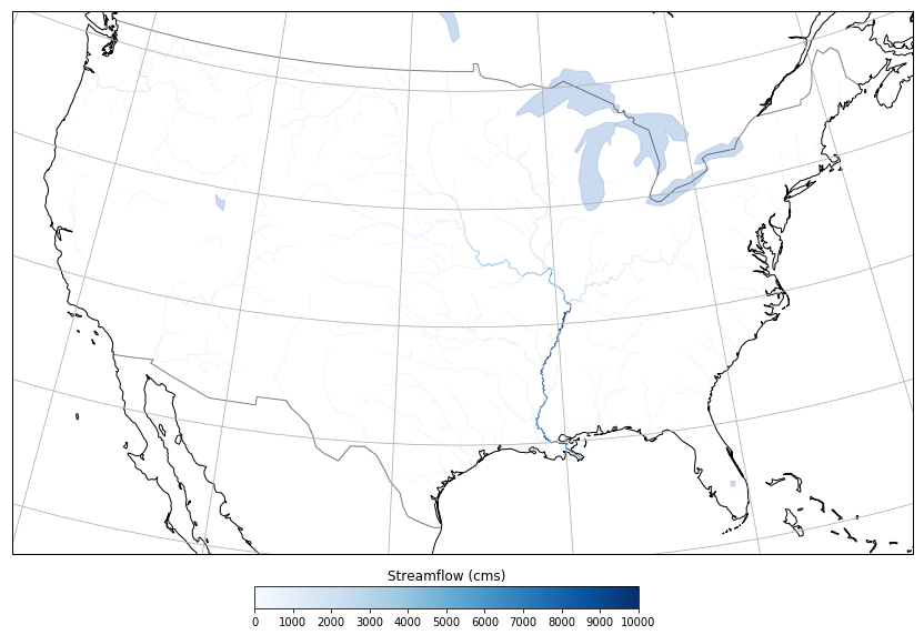
Now that we have the shapefile with the flow segments loaded lets plot the streamflow onto a map. To do this we need to join the feature ids in the model output the streamflow values in the model output. We do this by performing a dictionary comphrension to map feature ids and streamflow values together.
CHRTOUT = Dataset('201409090000.CHRTOUT_DOMAIN1.comp', 'r')
feature_ids = CHRTOUT.variables['feature_id']
flows = CHRTOUT.variables['streamflow']
feature_idsa = np.array(feature_ids)
flowsa = np.array(flows)
streamflow = {key: value for (key, value) in zip(feature_idsa, flowsa)}
Now that we have a dictionary of segment ids and streamflow values we can map each flow line segment to its appropriate streamflow value. We also need to set the colors for each segment based on the value of the streamflow. We do that below with a helper function that combines both steps.
colorBarMin = 0.0
colorBarMax = 10000.0
colorMap = "Blues"
CMap = MplColorHelper(colorMap, colorBarMin, colorBarMax)

def GetStreamflowColor(info):
    key = info['COMID']
    if key in streamflow:
        return CMap.get_rgb(streamflow[key])
    return (0.0, 0.0, 0.0, 0.0)

flowline_streamflow_color = [GetStreamflowColor(line['properties']) for line in shp_10k]
Now that we have the color we want to plot each segment in we can make the figure. This is very similar to what we did above but now mapping in the color based on streamflow for each flow line segment.
lccProjParams = { 'central_latitude'   : 50.0, # same as lat_0 in proj4 string
                  'central_longitude'  : -96.0, # same as lon_0
                  'standard_parallels' : (33.0, 45.0) # same as (lat_1, lat_2)
}
proj = ccrs.LambertConformal(**lccProjParams)

fig = plt.figure(figsize=(16,9))
ax = plt.axes(projection = proj)
ax.set_extent([-120.0, -72.0, 22.0, 50.0])

# we add edgecolor = here to set the colors based on streamflow
ax.add_feature(feature.ShapelyFeature(mp_10k, shpProj),
        edgecolor = flowline_streamflow_color)

ax.add_feature(feature.NaturalEarthFeature(
        category='cultural',
        name='admin_1_states_provinces_lines',
        scale='50m',
        facecolor='none'))
ax.add_feature(feature.NaturalEarthFeature(
        category='physical',
        name='lakes',
        scale='50m',
        facecolor='none'))
ax.coastlines('50m')
ax.add_feature(feature.LAKES, alpha=0.5)
ax.add_feature(feature.BORDERS, linestyle='-', alpha=.5)
ax.gridlines()

# We also add a legend here to relate the streamflow colors to values
ax_legend = fig.add_axes([0.35, 0.05, 0.3, 0.03], zorder=3)
ticks = np.arange(colorBarMin,colorBarMax+0.5,1000.0)
cb = matplotlib.colorbar.ColorbarBase(ax_legend, cmap=colorMap, ticks=ticks, norm=matplotlib.colors.Normalize(vmin=colorBarMin, vmax=colorBarMax), orientation='horizontal')
cb.ax.set_xticklabels([str(int(i)) for i in ticks])

plt.title('Streamflow (cms)')
Text(0.5,1,'Streamflow (cms)')
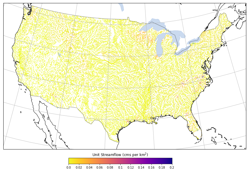
Unit Streamflow
We can see the Mississippi River dominates the visualization of the streamflow values. Just what we would expect given the land mass that the river drains!
However, flooding is relative to the capacity for each segment of a given stream. One way to visualize anomalous values better is to normalize each segment by the drainage area. We show an example of how to compute the unit streamflow (streamflow per square kilometer of drained land mass).
Because this is most useful for identifying floods in small drainage areas we will switch to using the shapefile we created with all drainage areas over 100 square kilometers.
colorBarMin = 0.0
colorBarMax = 0.2
colorMap = "plasma_r"
CMap = MplColorHelper(colorMap, colorBarMin, colorBarMax)

def GetUnitStreamflowColor(info):
    key = info['COMID']
    if key in streamflow:
        return CMap.get_rgb(streamflow[key] / info['TotDASqKm'])
    return (0.0, 0.0, 0.0, 0.0)


flowline_unitstreamflow_color = [GetUnitStreamflowColor(line['properties']) for line in shp_100]
Above we repeat the process of mapping the flow lines to a color, this time dividing the streamflow by the drainage area. We separate out these steps into different cells because of the computation time both take. It is easier to not have to repeat the entire process if you only want to change something with the figure for example.
lccProjParams = { 'central_latitude'   : 50.0, # same as lat_0 in proj4 string
                  'central_longitude'  : -96.0, # same as lon_0
                  'standard_parallels' : (33.0, 45.0) # same as (lat_1, lat_2)
}
proj = ccrs.LambertConformal(**lccProjParams)

fig = plt.figure(figsize=(16,9))
ax = plt.axes(projection = proj)
ax.set_extent([-120.0, -72.0, 22.0, 50.0])
ax.add_feature(feature.ShapelyFeature(mp_100, shpProj),
        edgecolor = flowline_unitstreamflow_color)
ax.add_feature(feature.NaturalEarthFeature(
        category='cultural',
        name='admin_1_states_provinces_lines',
        scale='50m',
        facecolor='none'))
ax.add_feature(feature.NaturalEarthFeature(
        category='physical',
        name='lakes',
        scale='50m',
        facecolor='none'))
ax.coastlines('50m')
ax.add_feature(feature.LAKES, alpha=0.5)
ax.add_feature(feature.BORDERS, linestyle='-', alpha=.5)
ax.gridlines()
ax_legend = fig.add_axes([0.35, 0.05, 0.3, 0.03], zorder=3)
ticks = np.arange(colorBarMin,colorBarMax+0.5,0.02)
cb = matplotlib.colorbar.ColorbarBase(ax_legend, cmap=colorMap, ticks=ticks, norm=matplotlib.colors.Normalize(vmin=colorBarMin, vmax=colorBarMax), orientation='horizontal')
cb.ax.set_xticklabels([str(round(i,2)) for i in ticks])
plt.title('Unit Streamflow (cms per km$^2$)')
Text(0.5,1,'Unit Streamflow (cms per km$^2$)')
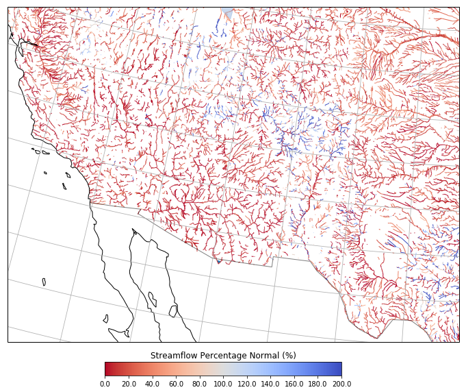
Streamflow Normals
We can alternatively normalize the streamflow values by comparing to the mean over a long period of record. We will show how that is done here using the EROM values from the NHDPlus dataset.
colorBarMin = 0.0
colorBarMax = 200.0
colorMap = "coolwarm_r"
CMap = MplColorHelper(colorMap, colorBarMin, colorBarMax)

def GetRelativeStreamflowColor(info):
    key = info['COMID']
    if key in streamflow and info['QE_MA'] > 0.0:
        return CMap.get_rgb(streamflow[key] / (info['QE_MA'] * 0.0283168) * 100.0)
    return (0.0, 0.0, 0.0, 0.0)


flowline_relativestreamflow_color = [GetRelativeStreamflowColor(line['properties']) for line in shp_100]
And we will repeat the plotting exercise one more time this time zooming in on the southwest United States.
lccProjParams = { 'central_latitude'   : 50.0, # same as lat_0 in proj4 string
                  'central_longitude'  : -96.0, # same as lon_0
                  'standard_parallels' : (33.0, 45.0) # same as (lat_1, lat_2)
}
proj = ccrs.LambertConformal(**lccProjParams)

fig = plt.figure(figsize=(16,9))
ax = plt.axes(projection = proj)
ax.set_extent([-120.0, -100.0, 29.0, 40.0])
ax.add_feature(feature.ShapelyFeature(mp_100, shpProj),
        edgecolor = flowline_relativestreamflow_color)
ax.add_feature(feature.NaturalEarthFeature(
        category='cultural',
        name='admin_1_states_provinces_lines',
        scale='50m',
        facecolor='none'))
ax.add_feature(feature.NaturalEarthFeature(
        category='physical',
        name='lakes',
        scale='50m',
        facecolor='none'))
ax.coastlines('50m')
ax.add_feature(feature.LAKES, alpha=0.5)
ax.add_feature(feature.BORDERS, linestyle='-', alpha=.5)
ax.gridlines()
ax_legend = fig.add_axes([0.35, 0.05, 0.3, 0.03], zorder=3)
ticks = np.arange(colorBarMin,colorBarMax+0.5,20.0)
cb = matplotlib.colorbar.ColorbarBase(ax_legend, cmap=colorMap, ticks=ticks, norm=matplotlib.colors.Normalize(vmin=colorBarMin, vmax=colorBarMax), orientation='horizontal')
cb.ax.set_xticklabels([str(round(i,2)) for i in ticks])
plt.title('Streamflow Percentage Normal (%)')
Text(0.5,1,'Streamflow Percentage Normal (%)')
Jupyter Notebook
The notebook and example data shown here are available at https://github.com/occ-data/nwm-jupyter